what the Dunning-Kruger effect is and isn’t

If you regularly read cognitive science or psychology blogs (or even just the lowly New York Times!), you’ve probably heard of something called the Dunning-Kruger effect. The Dunning-Kruger effect refers to the seemingly pervasive tendency of poor performers to overestimate their abilities relative to other people–and, to a lesser extent, for high performers to underestimate their abilities. The explanation for this, according to Kruger and Dunning, who first reported the effect in an extremely influential 1999 article in the Journal of Personality and Social Psychology, is that incompetent people by lack the skills they’d need in order to be able to distinguish good performers from bad performers:

…people who lack the knowledge or wisdom to perform well are often unaware of this fact. We attribute this lack of awareness to a deficit in metacognitive skill. That is, the same incompetence that leads them to make wrong choices also deprives them of the savvy necessary to recognize competence, be it their own or anyone else’s.

For reasons I’m not really clear on, the Dunning-Kruger effect seems to be experiencing something of a renaissance over the past few months; it’s everywhere in the blogosphere and media. For instance, here are just a few alleged Dunning-Krugerisms from the past few weeks:

So what does this mean in business? Well, it’s all over the place. Even the title of Dunning and Kruger’s paper, the part about inflated self-assessments, reminds me of a truism that was pointed out by a supervisor early in my career: The best employees will invariably be the hardest on themselves in self-evaluations, while the lowest performers can be counted on to think they are doing excellent work…

Heidi Montag and Spencer Pratt are great examples of the Dunning-Kruger effect. A whole industry of assholes are making a living off of encouraging two attractive yet untalented people they are actually genius auteurs. The bubble around them is so thick, they may never escape it. At this point, all of America (at least those who know who they are), is in on the joke ““ yet the two people in the center of this tragedy are completely unaware…

Not so fast there — the Dunning-Kruger effect comes into play here. People in the United States do not have a high level of understanding of evolution, and this survey did not measure actual competence. I’ve found that the people most likely to declare that they have a thorough knowledge of evolution are the creationists“¦but that a brief conversation is always sufficient to discover that all they’ve really got is a confused welter of misinformation…

As you can see, the findings reported by Kruger and Dunning are often interpreted to suggest that the less competent people are, the more competent they think they are. People who perform worst at a task tend to think they’re god’s gift to said task, and the people who can actually do said task often display excessive modesty. I suspect we find this sort of explanation compelling because it appeals to our implicit just-world theories: we’d like to believe that people who obnoxiously proclaim their excellence at X, Y, and Z must really not be so very good at X, Y, and Z at all, and must be (over)compensating for some actual deficiency; it’s much less pleasant to imagine that people who go around shoving their (alleged) superiority in our faces might really be better than us at what they do.

Unfortunately, Kruger and Dunning never actually provided any support for this type of just-world view; their studies categorically didn’t show that incompetent people are more confident or arrogant than competent people. What they did show is this:

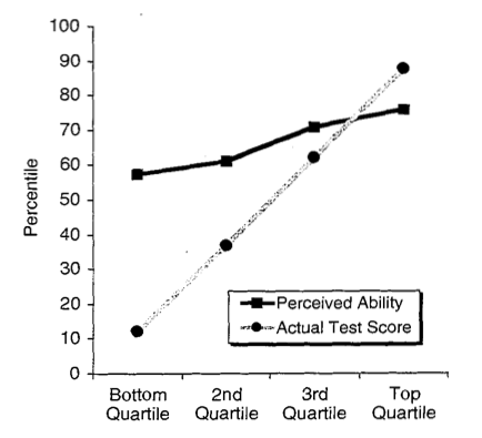
This is one of the key figures from Kruger and Dunning’s 1999 paper (and the basic effect has been replicated many times since). The critical point to note is that there’s a clear positive correlation between actual performance (gray line) and perceived performance (black line): the people in the top quartile for actual performance think they perform better than the people in the second quartile, who in turn think they perform better than the people in the third quartile, and so on. So the bias is definitively not that incompetent people think they’re better than competent people. Rather, it’s that incompetent people think they’re much better than they actually are. But they typically still don’t think they’re quite as good as people who, you know, actually are good. (It’s important to note that Dunning and Kruger never claimed to show that the unskilled think they’re better than the skilled; that’s just the way the finding is often interpreted by others.)

That said, it’s clear that there is a very large discrepancy between the way incompetent people actually perform and the way they perceive their own performance level, whereas the discrepancy is much smaller for highly competent individuals. So the big question is why. Kruger and Dunning’s explanation, as I mentioned above, is that incompetent people lack the skills they’d need in order to know they’re incompetent. For example, if you’re not very good at learning languages, it might be hard for you to tell that you’re not very good, because the very skills that you’d need in order to distinguish someone who’s good from someone who’s not are the ones you lack. If you can’t hear the distinction between two different phonemes, how could you ever know who has native-like pronunciation ability and who doesn’t? If you don’t understand very many words in another language, how can you evaluate the size of your own vocabulary in relation to other people’s?

This appeal to people’s meta-cognitive abilities (i.e., their knowledge about their knowledge) has some intuitive plausibility, and Kruger, Dunning and their colleagues have provided quite a bit of evidence for it over the past decade. That said, it’s by no means the only explanation around; over the past few years, a fairly sizeable literature criticizing or extending Kruger and Dunning’s work has developed. I’ll mention just three plausible (and mutually compatible) alternative accounts people have proposed (but there are others!)

1. Regression toward the mean. Probably the most common criticism of the Dunning-Kruger effect is that it simply reflects regression to the mean–that is, it’s a statistical artifact. Regression to the mean refers to the fact that any time you select a group of individuals based on some criterion, and then measure the standing of those individuals on some other dimension, performance levels will tend to shift (or regress) toward the mean level. It’s a notoriously underappreciated problem, and probably explains many, many phenomena that people have tried to interpret substantively. For instance, in placebo-controlled clinical trials of SSRIs, depressed people tend to get better in both the drug and placebo conditions. Some of this is undoubtedly due to the placebo effect, but much of it is probably also due to what’s often referred to as “natural history”. Depression, like most things, tends to be cyclical: people get better or worse better over time, often for no apparent rhyme or reason. But since people tend to seek help (and sign up for drug trials) primarily when they’re doing particularly badly, it follows that most people would get better to some extent even without any treatment. That’s regression to the mean (the Wikipedia entry has other nice examples–for example, the famous Sports Illustrated Cover Jinx).

In the context of the Dunning-Kruger effect, the argument is that incompetent people simply regress toward the mean when you ask them to evaluate their own performance. Since perceived performance is influenced not only by actual performance, but also by many other factors (e.g., one’s personality, meta-cognitive ability, measurement error, etc.), it follows that, on average, people with extreme levels of actual performance won’t be quite as extreme in terms of their perception of their performance. So, much of the Dunning-Kruger effect arguably doesn’t need to be explained at all, and in fact, it would be quite surprising if you didn’t see a pattern of results that looks at least somewhat like the figure above.

2. Regression to the mean plus better-than-average. Having said that, it’s clear that regression to the mean can’t explain everything about the Dunning-Kruger effect. One problem is that it doesn’t explain why the effect is greater at the low end than at the high end. That is, incompetent people tend to overestimate their performance to a much greater extent than competent people underestimate their performance. This asymmetry can’t be explained solely by regression to the mean. It can, however, be explained by a combination of RTM and a “better-than-average” (or self-enhancement) heuristic which says that, in general, most people have a tendency to view themselves excessively positively. This two-pronged explanation was proposed by Krueger and Mueller in a 2002 study (note that Krueger and Kruger are different people!), who argued that poor performers suffer from a double whammy: not only do their perceptions of their own performance regress toward the mean, but those perceptions are also further inflated by the self-enhancement bias. In contrast, for high performers, these two effects largely balance each other out: regression to the mean causes high performers to underestimate their performance, but to some extent that underestimation is offset by the self-enhancement bias. As a result, it looks as though high performers make more accurate judgments than low performers, when in reality the high performers are just lucky to be where they are in the distribution.

3. The instrumental role of task difficulty. Consistent with the notion that the Dunning-Kruger effect is at least partly a statistical artifact, some studies have shown that the asymmetry reported by Kruger and Dunning (i.e., the smaller discrepancy for high performers than for low performers) actually goes away, and even reverses, when the ability tests given to participants are very difficult. For instance, Burson and colleagues (2006), writing in JPSP, showed that when University of Chicago undergraduates were asked moderately difficult trivia questions about their university, the subjects who performed best were just as poorly calibrated as the people who performed worst, in the sense that their estimates of how well they did relative to other people were wildly inaccurate. Here’s what that looks like:

Notice that this finding wasn’t anomalous with respect to the Kruger and Dunning findings; when participants were given easier trivia (the diamond-studded line), Burson et al observed the standard pattern, with poor performers seemingly showing worse calibration. Simply knocking about 10% off the accuracy rate on the trivia questions was enough to induce a large shift in the relative mismatch between perceptions of ability and actual ability. Burson et al then went on to replicate this pattern in two additional studies involving a number of different judgments and tasks, so this result isn’t specific to trivia questions. In fact, in the later studies, Burson et al showed that when the task was really difficult, poor performers were actually considerably better calibrated than high performers.

Looking at the figure above, it’s not hard to see why this would be. Since the slope of the line tends to be pretty constant in these types of experiments, any change in mean performance levels (i.e., a shift in intercept on the y-axis) will necessarily result in a larger difference between actual and perceived performance at the high end. Conversely, if you raise the line, you maximize the difference between actual and perceived performance at the lower end.

To get an intuitive sense of what’s happening here, just think of it this way: if you’re performing a very difficult task, you’re probably going to find the experience subjectively demanding even if you’re at the high end relative to other people. Since people’s judgments about their own relative standing depends to a substantial extent on their subjective perception of their own performance (i.e., you use your sense of how easy a task was as a proxy of how good you must be at it), high performers are going to end up systematically underestimating how well they did. When a task is difficult, most people assume they must have done relatively poorly compared to other people. Conversely, when a task is relatively easy (and the tasks Dunning and Kruger studied were on the easier side), most people assume they must be pretty good compared to others. As a result, it’s going to look like the people who perform well are well-calibrated when the task is easy and poorly-calibrated when the task is difficult; less competent people are going to show exactly the opposite pattern. And note that this doesn’t require us to assume any relationship between actual performance and perceived performance. You would expect to get the Dunning-Kruger effect for easy tasks even if there was exactly zero correlation between how good people actually are at something and how good they think they are.

Here’s how Burson et al summarized their findings:

Our studies replicate, eliminate, or reverse the association between task performance and judgment accuracy reported by Kruger and Dunning (1999) as a function of task difficulty. On easy tasks, where there is a positive bias, the best performers are also the most accurate in estimating their standing, but on difficult tasks, where there is a negative bias, the worst performers are the most accurate. This pattern is consistent with a combination of noisy estimates and overall bias, with no need to invoke differences in metacognitive abilities. In this  regard, our findings support Krueger and Mueller’s (2002) reinterpretation of Kruger and Dunning’s (1999) findings. An association between task-related skills and metacognitive insight may indeed exist, and later we offer some suggestions for ways to test for it. However, our analyses indicate that the primary drivers of errors in judging relative standing are general inaccuracy and overall biases tied to task difficulty. Thus, it is important to know more about those sources of error in order to better understand and ameliorate them.

What should we conclude from these (and other) studies? I think the jury’s still out to some extent, but at minimum, I think it’s clear that much of the Dunning-Kruger effect reflects either statistical artifact (regression to the mean), or much more general cognitive biases (the tendency to self-enhance and/or to use one’s subjective experience as a guide to one’s standing in relation to others). This doesn’t mean that the meta-cognitive explanation preferred by Dunning, Kruger and colleagues can’t hold in some situations; it very well may be that in some cases, and to some extent, people’s lack of skill is really what prevents them from accurately determining their standing in relation to others. But I think our default position should be to prefer the alternative explanations I’ve discussed above, because they’re (a) simpler, (b) more general (they explain lots of other phenomena), and (c) necessary (frankly, it’d be amazing if regression to the mean didn’t explain at least part of the effect!).

We should also try to be aware of another very powerful cognitive bias whenever we use the Dunning-Kruger effect to explain the people or situations around us–namely, confirmation bias. If you believe that incompetent people don’t know enough to know they’re incompetent, it’s not hard to find anecdotal evidence for that; after all, we all know people who are both arrogant and not very good at what they do. But if you stop to look for it, it’s probably also not hard to find disconfirming evidence. After all, there are clearly plenty of people who are good at what they do, but not nearly as good as they think they are (i.e., they’re above average, and still totally miscalibrated in the positive direction). Just like there are plenty of people who are lousy at what they do and recognize their limitations (e.g., I don’t need to be a great runner in order to be able to tell that I’m not a great runner–I’m perfectly well aware that I have terrible endurance, precisely because I can’t finish runs that most other runners find trivial!). But the plural of anecdote is not data, and the data appear to be equivocal. Next time you’re inclined to chalk your obnoxious co-worker’s delusions of grandeur down to the Dunning-Kruger effect, consider the possibility that your co-worker’s simply a jerk–no meta-cognitive incompetence necessary.

ResearchBlogging.orgKruger J, & Dunning D (1999). Unskilled and unaware of it: how difficulties in recognizing one’s own incompetence lead to inflated self-assessments. Journal of personality and social psychology, 77 (6), 1121-34 PMID: 10626367
Krueger J, & Mueller RA (2002). Unskilled, unaware, or both? The better-than-average heuristic and statistical regression predict errors in estimates of own performance. Journal of personality and social psychology, 82 (2), 180-8 PMID: 11831408
Burson KA, Larrick RP, & Klayman J (2006). Skilled or unskilled, but still unaware of it: how perceptions of difficulty drive miscalibration in relative comparisons. Journal of personality and social psychology, 90 (1), 60-77 PMID: 16448310

fourteen questions about selection bias, circularity, nonindependence, etc.

A new paper published online this week in the Journal of Cerebral Blood Flow & Metabolism this week discusses the infamous problem of circular analysis in fMRI research. The paper is aptly titled “Everything you never wanted to know about circular analysis, but were afraid to ask,” and is authored by several well-known biostatisticians and cognitive neuroscientists–to wit, Niko Kriegeskorte, Martin Lindquist, Tom Nichols, Russ Poldrack, and Ed Vul. The paper has an interesting format, and one that I really like: it’s set up as a series of fourteen questions related to circular analysis, and each author answers each question in 100 words or less.

I won’t bother going over the gist of the paper, because the Neuroskeptic already beat me to the punch in an excellent post a couple of days ago (actually, that’s how I found out about the paper); instead,  I’ll just give my own answers to the same set of questions raised in the paper. And since blog posts don’t have the same length constraints as NPG journals, I’m going to be characteristically long-winded and ignore the 100 word limit…

(1) Is circular analysis a problem in systems and cognitive neuroscience?

Yes, it’s a huge problem. That said, I think the term ‘circular’ is somewhat misleading here, because it has the connotation than an analysis is completely vacuous. Truly circular analyses–i.e., those where an initial analysis is performed, and the researchers then conduct a “follow-up” analysis that literally adds no new information–are relatively rare in fMRI research. Much more common are cases where there’s some dependency between two different analyses, but the second one still adds some novel information.

(2) How widespread are slight distortions and serious errors caused by circularity in the neuroscience literature?

I think Nichols sums it up nicely here:

TN: False positives due to circularity are minimal; biased estimates of effect size are common. False positives due to brushing off the multiple testing problem (e.g., “˜P<0.001 uncorrected’ and crossing your fingers) remain pervasive.

The only thing I’d add to this is that the bias in effect size estimates is not only common, but, in most cases, is probably very large.

(3) Are circular estimates useful measures of effect size?

Yes and no. They’re less useful than unbiased measures of effect size. But given that the vast majority of effects reported in whole-brain fMRI analyses (and, more generally, analyses in most fields) are likely to be inflated to some extent, the only way to ensure we don’t rely on circular estimates of effect size would be to disregard effect size estimates entirely, which doesn’t seem prudent.

(4) Should circular estimates of effect size be presented in papers and, if so, how?

Yes, because the only principled alternatives are to either (a) never report effect sizes (which seems much too drastic), or (b) report the results of every single test performed, irrespective of the result (i.e., to never give selection bias an opportunity to rear its head). Neither of these is reasonable. We should generally report effect sizes for all key effects, but they should be accompanied by appropriate confidence intervals. As Lindquist notes:

In general, it may be useful to present any effect size estimate as confidence intervals, so that readers can see for themselves how much uncertainty is related to the point estimate.

A key point I’d add is that the width of the reported CIs should match the threshold used to identify results in the first place. In other words, if you conduct a whole brain analysis at p < .001, you should report all resulting effects with 99.9% CIs, and not 95% CIs. I think this simple step would go a considerable ways towards conveying the true uncertainty surrounding most point estimates in fMRI studies.

(5) Are effect size estimates important/useful for neuroscience research, and why?

I think my view here is closest to Ed Vul’s:

Yes, very much so. Null-hypothesis testing is insufficient for most goals of neuroscience because it can only indicate that a brain region is involved to some nonzero degree in some task contrast. This is likely to be true of most combinations of task contrasts and brain regions when measured with sufficient power.

I’d go further than Ed does though, and say that in a sense, effect size estimates are the only things that matter. As Ed notes, there are few if any cases where it’s plausible to suppose that the effect of some manipulation on brain activation is really zero. The brain is a very dense causal system–almost any change in one variable is going to have downstream effects on many, and perhaps most, others. So the real question we care about is almost never “is there or isn’t there an effect,” it’s whether there’s an effect that’s big enough to actually care about. (This problem isn’t specific to fMRI research, of course; it’s been a persistent source of criticism of null hypothesis significance testing for many decades.)

People sometimes try to deflect this concern by saying that they’re not trying to make any claims about how big an effect is, but only about whether or not one can reject the null–i.e., whether any kind of effect is present or not. I’ve never found this argument convincing, because whether or not you own up to it, you’re always making an effect size claim whenever you conduct a hypothesis test. Testing against a null of zero is equivalent to saying that you care about any effect that isn’t exactly zero, which is simply false. No one in fMRI research cares about r or d values of 0.0001, yet we routinely conduct tests whose results could be consistent with those types of effect sizes.

Since we’re always making implicit claims about effect sizes when we conduct hypothesis tests, we may as well make them explicit so that they can be evaluated properly. If you only care about correlations greater than 0.1, there’s no sense in hiding that fact; why not explicitly test against a null range of -0.1 to 0.1, instead of a meaningless null of zero?

(6) What is the best way to accurately estimate effect sizes from imaging data?

Use large samples, conduct multivariate analyses, report results comprehensively, use meta-analysis… I don’t think there’s any single way to ensure accurate effect size estimates, but plenty of things help. Maybe the most general recommendation is to ensure adequate power (see below), which will naturally minimize effect size inflation.

(7) What makes data sets independent? Are different sets of subjects required?

Most of the authors think (as I do too) that different sets of subjects are indeed required in order to ensure independence. Here’s Nichols:

Only data sets collected on distinct individuals can be assured to be independent. Splitting an individual’s data (e.g., using run 1 and run 2 to create two data sets) does not yield independence at the group level, as each subject’s true random effect will correlate the data sets.

Put differently, splitting data within subjects only eliminates measurement error, and not sampling error. You could in theory measure activation perfectly reliably (in which case the two halves of subjects’ data would be perfectly correlated) and still have grossly inflated effects, simply because the multivariate distribution of scores in your sample doesn’t accurately reflect the distribution in the population. So, as Nichols points out, you always need new subjects if you want to be absolutely certain your analyses are independent. But since this generally isn’t feasible, I’d argue we should worry less about whether or not our data sets are completely independent, and more about reporting results in a way that makes the presence of any bias as clear as possible.

(8) What information can one glean from data selected for a certain effect?

I think this is kind of a moot question, since virtually all data are susceptible to some form of selection bias (scientists generally don’t write papers detailing all the analyses they conducted that didn’t pan out!). As I note above, I think it’s a bad idea to disregard effect sizes entirely; they’re actually what we should be focusing most of our attention on. Better to report confidence intervals that accurately reflect the selection procedure and make the uncertainty around the point estimate clear.

(9) Are visualizations of nonindependent data helpful to illustrate the claims of a paper?

Not in cases where there’s an extremely strong dependency between the selection criteria and the effect size estimate. In cases of weak to moderate dependency, visualization is fine so long as confidence bands are plotted alongside the best fit. Again, the key is to always be explicit about the limitations of the analysis and provide some indication of the uncertainty involved.

(10) Should data exploration be discouraged in favor of valid confirmatory analyses?

No. I agree with Poldrack’s sentiment here:

Our understanding of brain function remains incredibly crude, and limiting research to the current set of models and methods would virtually guarantee scientific failure. Exploration of new approaches is thus critical, but the findings must be confirmed using new samples and convergent methods.

(11) Is a confirmatory analysis safer than an exploratory analysis in terms of drawing neuroscientific conclusions?

In principle, sure, but in practice, it’s virtually impossible to determine which reported analyses really started out their lives as confirmatory analyses and which started life out as exploratory analyses and then mysteriously evolved into “a priori” predictions once the paper was written. I’m not saying there’s anything wrong with this–everyone reports results strategically to some extent–just that I don’t know that the distinction between confirmatory and exploratory analyses is all that meaningful in practice. Also, as the previous point makes clear, safety isn’t the only criterion we care about; we also want to discover new and unexpected findings, which requires exploration.

(12) What makes a whole-brain mapping analysis valid? What constitutes sufficient adjustment for multiple testing?

From a hypothesis testing standpoint, you need to ensure adequate control of the family-wise error (FWE) rate or false discovery rate (FDR). But as I suggested above, I think this only ensures validity in a limited sense; it doesn’t ensure that the results are actually going to be worth caring about. If you want to feel confident that any effects that survive are meaningfully large, you need to do the extra work up front and define what constitutes a meaningful effect size (and then test against that).

(13) How much power should a brain-mapping analysis have to be useful?

As much as possible! Concretely, the conventional target of 80% seems like a good place to start. But as I’ve argued before (e.g., here), that would require more than doubling conventional sample sizes in most cases. The reality is that fMRI studies are expensive, so we’re probably stuck with underpowered analyses for the foreseeable future. So we need to find other ways to compensate for that (e.g., relying more heavily on meta-analytic effect size estimates).

(14) In which circumstances are nonindependent selective analyses acceptable for scientific publication?

It depends on exactly what’s problematic about the analysis. Analyses that are truly circular and provide no new information should never be reported, but those constitute only a small fraction of all analyses. More commonly, the nonindependence simply amounts to selection bias: researchers tend to report only those results that achieve statistical significance, thereby inflating apparent effect sizes. I think the solution to this is to still report all key effect sizes, but to ensure they’re accompanied by confidence intervals and appropriate qualifiers.

ResearchBlogging.orgKriegeskorte N, Lindquist MA, Nichols TE, Poldrack RA, & Vul E (2010). Everything you never wanted to know about circular analysis, but were afraid to ask. Journal of cerebral blood flow and metabolism : official journal of the International Society of Cerebral Blood Flow and Metabolism PMID: 20571517

the capricious nature of p < .05, or why data peeking is evil

There’s a time-honored tradition in the social sciences–or at least psychology–that goes something like this. You decide on some provisional number of subjects you’d like to run in your study; usually it’s a nice round number like twenty or sixty, or some number that just happens to coincide with the sample size of the last successful study you ran. Or maybe it just happens to be your favorite number (which of course is forty-four). You get your graduate student to start running the study, and promptly forget about it for a couple of weeks while you go about writing up journal reviews that are three weeks overdue and chapters that are six months overdue.

A few weeks later, you decide you’d like to know how that Amazing New Experiment you’re running is going. You summon your RA and ask him, in magisterial tones, “how’s that Amazing New Experiment we’re running going?” To which he falteringly replies that he’s been very busy with all the other data entry and analysis chores you assigned him, so he’s only managed to collect data from eighteen subjects so far. But he promises to have the other eighty-two subjects done any day now.

“Not to worry,” you say. “We’ll just take a peek at the data now and see what it looks like; with any luck, you won’t even need to run any more subjects! By the way, here are my car keys; see if you can’t have it washed by 5 pm. Your job depends on it. Ha ha.”

Once your RA’s gone to soil himself somewhere, you gleefully plunge into the task of peeking at your data. You pivot your tables, plyr your data frame, and bravely sort your columns. Then you extract two of the more juicy variables for analysis, and after some careful surgery a t-test or six, you arrive at the conclusion that your hypothesis is… “marginally” supported. Which is to say, the magical p value is somewhere north of .05 and somewhere south of .10, and now it’s just parked by the curb waiting for you to give it better directions.

You briefly contemplate reporting your result as a one-tailed test–since it’s in the direction you predicted, right?–but ultimately decide against that. You recall the way your old Research Methods professor used to rail at length against the evils of one-sample tests, and even if you don’t remember exactly why they’re so evil, you’re not willing to take any chances. So you decide it can’t be helped; you need to collect some more data.

You summon your RA again. “Is my car washed yet?” you ask.

“No,” says your RA in a squeaky voice. “You just asked me to do that fifteen minutes ago.”

“Right, right,” you say. “I knew that.”

You then explain to your RA that he should suspend all other assigned duties for the next few days and prioritize running subjects in the Amazing New Experiment. “Abandon all other tasks!” you decree. “If it doesn’t involve collecting new data, it’s unimportant! Your job is to eat, sleep, and breathe new subjects! But not literally!”

Being quite clever, your RA sees an opening. “I guess you’ll want your car keys back, then,” he suggests.

“Nice try, Poindexter,” you say. “Abandon all other tasks… starting tomorrow.”

You also give your RA very careful instructions to email you the new data after every single subject, so that you can toss it into your spreadsheet and inspect the p value at every step. After all, there’s no sense in wasting perfectly good data; once your p value is below .05, you can just funnel the rest of the participants over to the Equally Amazing And Even Newer Experiment you’ve been planning to run as a follow-up. It’s a win-win proposition for everyone involved. Except maybe your RA, who’s still expected to return triumphant with a squeaky clean vehicle by 5 pm.

Twenty-six months and four rounds of review later, you publish the results of the Amazing New Experiment as Study 2 in a six-study paper in the Journal of Ambiguous Results. The reviewers raked you over the coals for everything from the suggested running head of the paper to the ratio between the abscissa and the ordinate in Figure 3. But what they couldn’t argue with was the p value in Study 2, which clocked in at just under p < .05, with only 21 subjects’ worth of data (compare that to the 80 you had to run in Study 4 to get a statistically significant result!). Suck on that, Reviewers!, you think to yourself pleasantly while driving yourself home from work in your shiny, shiny Honda Civic.

So ends our short parable, which has at least two subtle points to teach us. One is that it takes a really long time to publish anything; who has time to wait twenty-six months and go through four rounds of review?

The other, more important point, is that the desire to peek at one’s data, which often seems innocuous enough–and possibly even advisable (quality control is important, right?)–can actually be quite harmful. At least if you believe that the goal of doing research is to arrive at the truth, and not necessarily to publish statistically significant results.

The basic problem is that peeking at your data is rarely a passive process; most often, it’s done in the context of a decision-making process, where the goal is to determine whether or not you need to keep collecting data. There are two possible peeking outcomes that might lead you to decide to halt data collection: a very low p value (i.e., p < .05), in which case your hypothesis is supported and you may as well stop gathering evidence; or a very high p value, in which case you might decide that it’s unlikely you’re ever going to successfully reject the null, so you may as well throw in the towel. Either way, you’re making the decision to terminate the study based on the results you find in a provisional sample.

A complementary situation, which also happens not infrequently, occurs when you collect data from exactly as many participants as you decided ahead of time, only to find that your results aren’t quite what you’d like them to be (e.g., a marginally significant hypothesis test). In that case, it may be quite tempting to keep collecting data even though you’ve already hit your predetermined target. I can count on more than one hand the number of times I’ve overheard people say (often without any hint of guilt) something to the effect of “my p value’s at .06 right now, so I just need to collect data from a few more subjects.”

Here’s the problem with either (a) collecting more data in an effort to turn p < .06 into p < .05, or (b) ceasing data collection because you’ve already hit p < .05: any time you add another subject to your sample, there’s a fairly large probability the p value will go down purely by chance, even if there’s no effect. So there you are sitting at p < .06 with twenty-four subjects, and you decide to run a twenty-fifth subject. Well, let’s suppose that there actually isn’t a meaningful effect in the population, and that p < .06 value you’ve got is a (near) false positive. Adding that twenty-fifth subject can only do one of two things: it can raise your p value, or it can lower it. The exact probabilities of these two outcomes depends on the current effect size in your sample before adding the new subject; but generally speaking, they’ll rarely be very far from 50-50. So now you can see the problem: if you stop collecting data as soon as you get a significant result, you may well be capitalizing on chance. It could be that if you’d collected data from a twenty-sixth and twenty-seventh subject, the p value would reverse its trajectory and start rising. It could even be that if you’d collected data from two hundred subjects, the effect size would stabilize near zero. But you’d never know that if you stopped the study as soon as you got the results you were looking for.

Lest you think I’m exaggerating, and think that this problem falls into the famous class of things-statisticians-and-methodologists-get-all-anal-about-but-that-don’t-really-matter-in-the-real-world, here’s a sobering figure (taken from this chapter):

data_peeking

The figure shows the results of a simulation quantifying the increase in false positives associated with data peeking. The assumptions here are that (a) data peeking begins after about 10 subjects (starting earlier would further increase false positives, and starting later would decrease false positives somewhat), (b) the researcher stops as soon as a peek at the data reveals a result significant at p < .05, and (c) data peeking occurs at incremental steps of either 1 or 5 subjects. Given these assumptions, you can see that there’s a fairly monstrous rise in the actual Type I error rate (relative to the nominal rate of 5%). For instance, if the researcher initially plans to collect 60 subjects, but peeks at the data after every 5 subjects, there’s approximately a 17% chance that the threshold of p < .05 will be reached before the full sample of 60 subjects is collected. When data peeking occurs even more frequently (as might happen if a researcher is actively trying to turn p < .07 into p < .05, and is monitoring the results after each incremental participant), Type I error inflation is even worse. So unless you think there’s no practical difference between a 5% false positive rate and a 15 – 20% false positive rate, you should be concerned about data peeking; it’s not the kind of thing you just brush off as needless pedantry.

How do we stop ourselves from capitalizing on chance by looking at the data? Broadly speaking, there are two reasonable solutions. One is to just pick a number up front and stick with it. If you commit yourself to collecting data from exactly as many subjects as you said you would (you can proclaim the exact number loudly to anyone who’ll listen, if you find it helps), you’re then free to peek at the data all you want. After all, it’s not the act of observing the data that creates the problem; it’s the decision to terminate data collection based on your observation that matters.

The other alternative is to explicitly correct for data peeking. This is a common approach in large clinical trials, where data peeking is often ethically mandated, because you don’t want to either (a) harm people in the treatment group if the treatment turns out to have clear and dangerous side effects, or (b) prevent the control group from capitalizing on the treatment too if it seems very efficacious. In either event, you’d want to terminate the trial early. What researchers often do, then, is pick predetermined intervals at which to peek at the data, and then apply a correction to the p values that takes into account the number of, and interval between, peeking occasions. Provided you do things systematically in that way, peeking then becomes perfectly legitimate. Of course, the downside is that having to account for those extra inspections of the data makes your statistical tests more conservative. So if there aren’t any ethical issues that necessitate peeking, and you’re not worried about quality control issues that might be revealed by eyeballing the data, your best bet is usually to just pick a reasonable sample size (ideally, one based on power calculations) and stick with it.

Oh, and also, don’t make your RAs wash your car for you; that’s not their job.

Shalizi on the confounding of contagion and homophily in social network studies

Cosma Shalizi has a post up today discussing a new paper he wrote with Andrew C. Thomas arguing that it’s pretty much impossible to distinguish the effects of social contagion from homophily in observational studies.

That’s probably pretty cryptic without context, so here’s the background. A number of high-profile studies have been published in the past few years suggesting that everything from obesity to loneliness to pot smoking is socially contagious. The basic argument is that when you look at the diffusion of certain traits within social networks, you find that having friends who are obese is more likely to make you obese, having happy friends is more likely to make you happy, and so on. These effects (it’s been argued) persist even after you control for homophily–that is, the tendency of people to know and like other people who are similar to them–and can be indirect, so that you’re more likely to be obese even if your friends’ friends (who you may not even know know) are obese.

Needless to say, the work has been controversial. A few weeks ago, Dave Johns wrote an excellent pair of articles in Slate describing the original research, as well as the recent critical backlash (see also Andrew Gelman’s post here). Much of the criticism has focused on the question of whether it’s really possible to distinguish homophily from contagion using the kind of observational data and methods that contagion researchers have relied on. That is, if the probability that you’ll become obese (or lonely, or selfish, etc.) increases as a function of the number of obese people you know, is that because your acquaintance with obese people exerts a causal influence on your own body weight (e.g., by shaping your perception of body norms, eating habits, etc.), or is it simply that people with a disposition to become obese tend to seek out other people with the same disposition, and there’s no direct causal influence at all? It’s an important question, but one that’s difficult to answer conclusively.

In their new paper, Shalizi and Thomas use an elegant combination of logical argumentation, graphical causal models, and simulation to show that, in general, contagion effects are unidentifiable: you simply can’t tell whether like begets like because of a direct causal influence (“real” contagion), or because of homophily (birds of a feather flocking together). The only way out of the bind is to make unreasonably strong assumptions–e.g., that the covariates explicitly included in one’s model capture all of the influence of latent traits on observable behaviors. In his post Shalizi sums up the conclusions of the paper this way:

What the statistician or social scientist sees is that bridge-jumping is correlated across the social network. In this it resembles many, many, many behaviors and conditions, such as prescribing new antibiotics (one of the classic examples), adopting other new products, adopting political ideologies, attaching tags to pictures on flickr, attaching mis-spelled jokes to pictures of cats, smoking, drinking, using other drugs, suicide, literary tastes, coming down with infectious diseases, becoming obese, and having bad acne or being tall for your age. For almost all of these conditions or behaviors, our data is purely observational, meaning we cannot, for one reason or another, just push Joey off the bridge and see how Irene reacts. Can we nonetheless tell whether bridge-jumping spreads by (some form) of contagion, or rather is due to homophily, or, if it is both, say how much each mechanism contributes?

A lot of people have thought so, and have tried to come at it in the usual way, by doing regression. Most readers can probably guess what I think about that, so I will just say: don’t you wish. More sophisticated ideas, like propensity score matching, have also been tried, but people have pretty much assumed that it was possible to do this sort of decomposition. What Andrew and I showed is that in fact it isn’t, unless you are willing to make very strong, and generally untestable, assumptions.

It’s a very clear and compelling paper, and definitely worth reading if you have any interest at all in the question of whether and when it’s okay to apply causal modeling techniques to observational data. The answer Shalizi’s argued for on many occasions–and an unfortunate one from many scientists’ perspective–seems to be: very rarely if ever.

scientists aren’t dumb; statistics is hard

There’s a feature article in the new issue of Science News on the failure of science “to face the shortcomings of statistics”. The author, Tom Siegfried, argues that many scientific results shouldn’t be believed because they depend on faulty statistical practices:

Even when performed correctly, statistical tests are widely misunderstood and frequently misinterpreted. As a result, countless conclusions in the scientific literature are erroneous, and tests of medical dangers or treatments are often contradictory and confusing.

I have mixed feelings about the article. It’s hard to disagree with the basic idea that many scientific results are the results of statistical malpractice and/or misfortune. And Siegfried generally provides lucid explanations of some common statistical pitfalls when he sticks to the descriptive side of things. For instance, he gives nice accounts of Bayesian inference, of the multiple comparisons problem, and of the distinction between statistical significance and clinical/practical significance. And he nicely articulates what’s wrong with one of the most common (mis)interpretations of p values:

Correctly phrased, experimental data yielding a P value of .05 means that there is only a 5 percent chance of obtaining the observed (or more extreme) result if no real effect exists (that is, if the no-difference hypothesis is correct). But many explanations mangle the subtleties in that definition. A recent popular book on issues involving science, for example, states a commonly held misperception about the meaning of statistical significance at the .05 level: “This means that it is 95 percent certain that the observed difference between groups, or sets of samples, is real and could not have arisen by chance.“

So as a laundry list of common statistical pitfalls, it works quite nicely.

What I don’t really like about the article is that it seems to lay the blame squarely on the use of statistics to do science, rather than the way statistical analysis tends to be performed. That’s to say, a lay person reading the article could well come away with the impression that the very problem with science is that it relies on statistics. As opposed to the much more reasonable conclusion that science is hard, and statistics is hard, and ensuring that your work sits at the intersection of good science and good statistical practice is even harder. Siegfried all but implies that scientists are silly to base their conclusions on statistical inference. For instance:

It’s science’s dirtiest secret: The “scientific method“ of testing hypotheses by statistical analysis stands on a flimsy foundation. Statistical tests are supposed to guide scientists in judging whether an experimental result reflects some real effect or is merely a random fluke, but the standard methods mix mutually inconsistent philosophies and offer no meaningful basis for making such decisions.

Or:

Experts in the math of probability and statistics are well aware of these problems and have for decades expressed concern about them in major journals. Over the years, hundreds of published papers have warned that science’s love affair with statistics has spawned countless illegitimate findings. In fact, if you believe what you read in the scientific literature, you shouldn’t believe what you read in the scientific literature.

The problem is that there isn’t really any viable alternative to the “love affair with statistics”. Presumably Siegfried doesn’t think (most) scientists ought to be doing qualitative research; so the choice isn’t between statistics and no statistics, it’s between good and bad statistics.

In that sense, the tone of a lot of the article is pretty condescending: it comes off more like Siegfried saying “boy, scientists sure are dumb” and less like the more accurate observation that doing statistics is really hard, and it’s not surprising that even very smart people mess up frequently.

What makes it worse is that Siegfried slips up on a couple of basic points himself, and says some demonstrably false things in a couple of places. For instance, he explains failures to replicate genetic findings this way:

Nowhere are the problems with statistics more blatant than in studies of genetic influences on disease. In 2007, for instance, researchers combing the medical literature found numerous studies linking a total of 85 genetic variants in 70 different genes to acute coronary syndrome, a cluster of heart problems. When the researchers compared genetic tests of 811 patients that had the syndrome with a group of 650 (matched for sex and age) that didn’t, only one of the suspect gene variants turned up substantially more often in those with the syndrome — a number to be expected by chance.

“Our null results provide no support for the hypothesis that any of the 85 genetic variants tested is a susceptibility factor“ for the syndrome, the researchers reported in the Journal of the American Medical Association.

How could so many studies be wrong? Because their conclusions relied on “statistical significance,“ a concept at the heart of the mathematical analysis of modern scientific experiments.

This is wrong for at least two reasons. One is that, to believe the JAMA study Siegfried is referring to, and disbelieve the results of all 85 previously reported findings, you have to accept the null hypothesis, which is one of the very same errors Siegfried is supposed to be warning us against. In fact, you have to accept the null hypothesis 85 times. In the JAMA paper, the authors are careful to note that it’s possible the actual effects were simply overstated in the original studies, and that at least some of the original findings might still hold under more restrictive conditions. The conclusion that there really is no effect whatsoever is almost never warranted, because you rarely have enough power to rule out even very small effects. But Siegfried offers no such qualifiers; instead, he happily accepts 85 null hypotheses in support of his own argument.

The other issue is that it isn’t really the reliance on statistical significance that causes replication failures; it’s usually the use of excessively liberal statistical criteria. The problem has very little to do with the hypothesis testing framework per se. To see this, consider that if researchers always used a criterion of p < .0000001 instead of the conventional p < .05, there would almost never be any replication failures (because there would almost never be any statistically significant findings, period). So the problem is not so much with the classical hypothesis testing framework as with the choices many researchers make about how to set thresholds within that framework. (That’s not to say that there aren’t any problems associated with frequentist statistics, just that this isn’t really a fair one.)

Anyway, Siegfried’s explanations of the pitfalls of statistical significance then leads him to make what has to be hands-down the silliest statement in the article:

But in fact, there’s no logical basis for using a P value from a single study to draw any conclusion. If the chance of a fluke is less than 5 percent, two possible conclusions remain: There is a real effect, or the result is an improbable fluke. Fisher’s method offers no way to know which is which. On the other hand, if a study finds no statistically significant effect, that doesn’t prove anything, either. Perhaps the effect doesn’t exist, or maybe the statistical test wasn’t powerful enough to detect a small but real effect.

If you take this statement at face value, you should conclude there’s no point in doing statistical analysis, period. No matter what statistical procedure you use, you’re never going to know for cross-your-heart-hope-to-die sure that your conclusions are warranted. After all, you’re always going to have the same two possibilities: either the effect is real, or it’s not (or, if you prefer to frame the problem in terms of magnitude, either the effect is about as big as you think it is, or it’s very different in size). The same exact conclusion goes through if you take a threshold of p < .001 instead of one of p < .05: the effect can still be a spurious and improbable fluke. And it also goes through if you have twelve replications instead of just one positive finding: you could still be wrong (and people have been wrong). So saying that “two possible conclusions remain” isn’t offering any deep insight; it’s utterly vacuous.

The reason scientists use a conventional threshold of p < .05 when evaluating results isn’t because we think it gives us some magical certainty into whether a finding is “real” or not; it’s because it feels like a reasonable level of confidence to shoot for when making claims about whether the null hypothesis of no effect is likely to hold or not. Now there certainly are many problems associated with the hypothesis testing framework–some of them very serious–but if you really believe that “there’s no logical basis for using a P value from a single study to draw any conclusion,” your beef isn’t actually with p values, it’s with the very underpinnings of the scientific enterprise.

Anyway, the bottom line is Siegfried’s article is not so much bad as irresponsible. As an accessible description of some serious problems with common statistical practices, it’s actually quite good. But I guess the sense I got in reading the article was that at some point Siegfried became more interested in writing a contrarian piece about how scientists are falling down on the job than about how doing statistics well is just really hard for almost all of us (I certainly fail at it all the time!). And ironically, in the process of trying to explain just why “science fails to face the shortcomings of statistics”, Siegfried commits some of the very same errors he’s taking scientists to task for.

[UPDATE: Steve Novella says much the same thing here.]

[UPDATE 2: Andrew Gelman has a nice roundup of other comments on Siegfried’s article throughout the blogosphere.]

what the general factor of intelligence is and isn’t, or why intuitive unitarianism is a lousy guide to the neurobiology of higher cognitive ability

This post shamelessly plagiarizes liberally borrows ideas from a much longer, more detailed, and just generally better post by Cosma Shalizi. I’m not apologetic, since I’m a firm believer in the notion that good ideas should be repeated often and loudly. So I’m going to be often and loud here, though I’ll try to be (slightly) more succinct than Shalizi. Still, if you have the time to spare, you should read his longer and more mathematical take.

There’s a widely held view among intelligence researchers in particular, and psychologists more generally, that there’s a general factor of intelligence (often dubbed g) that accounts for a very large portion of the variance in a broad range of cognitive performance tasks. Which is to say, if you have a bunch of people do a bunch of different tasks, all of which we think tap different aspects of intellectual ability, and then you take all those scores and factor analyze them, you’ll almost invariably get a first factor that explains 50% or more of the variance in the zero-order scores. Or to put it differently, if you know a person’s relative standing on g, you can make a reasonable prediction about how that person will do on lots of different tasks–for example, digit symbol substitution, N-back, go/no-go, and so on and so forth. Virtually all tasks that we think reflect cognitive ability turn out, to varying extents, to reflect some underlying latent variable, and that latent variable is what we dub g.

In a trivial sense, no one really disputes that there’s such a thing as g. You can’t really dispute the existence of g, seeing as a general factor tends to fall out of virtually all factor analyses of cognitive tasks; it’s about as well-replicated a finding as you can get. To say that g exists, on the most basic reading, is simply to slap a name on the empirical fact that scores on different cognitive measures tend to intercorrelate positively to a considerable extent.

What’s not so clear is what the implications of g are for our understanding of how the human mind and brain works. If you take the presence of g at face value, all it really says is what we all pretty much already know: some people are smarter than others. People who do well in one intellectual domain will tend to do pretty well in others too, other things being equal. With the exception of some people who’ve tried to argue that there’s no such thing as general intelligence, but only “multiple intelligences” that totally fractionate across domains (not a compelling story, if you look at the evidence), it’s pretty clear that cognitive abilities tend to hang together pretty well.

The trouble really crops up when we try to say something interesting about the architecture of the human mind on the basis of the psychometric evidence for g. If someone tells you that there’s a single psychometric factor that explains at least 50% of the variance in a broad range of human cognitive abilities, it seems perfectly reasonable to suppose that that’s because there’s some unitary intelligence system in people’s heads, and that that system varies in capacity across individuals. In other words, the two intuitive models people have about intelligence seem to be that either (a) there’s some general cognitive system that corresponds to g, and supports a very large portion of the complex reasoning ability we call “intelligence” or (b) there are lots of different (and mostly unrelated) cognitive abilities, each of which contributes only to specific types of tasks and not others. Framed this way, it just seems obvious that the former view is the right one, and that the latter view has been discredited by the evidence.

The problem is that the psychometric evidence for g stems almost entirely from statistical procedures that aren’t really supposed to be use for causal inference. The primary weapon in the intelligence researcher’s toolbox has historically been principal components analysis (PCA) or exploratory factor analysis, which are really just data reduction techniques. PCA tells you how you can describe your data in a more compact way, but it doesn’t actually tell you what structure is in your data. A good analogy is the use of digital compression algorithms. If you take a directory full of .txt files and compress them into a single .zip file, you’ll almost certainly end up with a file that’s only a small fraction of the total size of the original texts. The reason this works is because certain patterns tend to repeat themselves over and over in .txt files, and a smart algorithm will store an abbreviated description of those patterns rather than the patterns themselves. Which, conceptually, is almost exactly what happens when you run a PCA on a dataset: you’re searching for consistent patterns in the way observations vary along multiple variables, and discarding any redundancy you come across in favor of a more compact description.

Now, in a very real sense, compression is impressive. It’s certainly nice to be able to email your friend a 140kb .zip of your 1200-page novel rather than a 2mb .doc. But note that you don’t actually learn much from the compression. It’s not like your friend can open up that 140k binary representation of your novel, read it, and spare herself the torture of the other 1860kb. If you want to understand what’s going on in a novel, you need to read the novel and think about the novel. And if you want to understand what’s going on in a set of correlations between different cognitive tasks, you need to carefully inspect those correlations and carefully think about those correlations. You can run a factor analysis if you like, and you might learn something, but you’re not going to get any deep insights into the “true” structure of the data. The “true” structure of the data is, by definition, what you started out with (give or take some error). When you run a PCA, you actually get a distorted (but simpler!) picture of the data.

To most people who use PCA, or other data reduction techniques, this isn’t a novel insight by any means. Most everyone who uses PCA knows that in an obvious sense you’re distorting the structure of the data when you reduce its dimensionality. But the use of data reduction is often defended by noting that there must be some reason why variables hang together in such a way that they can be reduced to a much smaller set of variables with relatively little loss of variance. In the context of intelligence, the intuition can be expressed as: if there wasn’t really a single factor underlying intelligence, why would we get such a strong first factor? After all, it didn’t have to turn out that way; we could have gotten lots of smaller factors that appear to reflect distinct types of ability, like verbal intelligence, spatial intelligence, perceptual speed, and so on. But it did turn out that way, so that tells us something important about the unitary nature of intelligence.

This is a strangely compelling argument, but it turns out to be only minimally true. What the presence of a strong first factor does tell you is that you have a lot of positively correlated variables in your data set. To be fair, that is informative. But it’s only minimally informative, because, assuming you eyeballed the correlation matrix in the original data, you already knew that.

What you don’t know, and can’t know, on the basis of a PCA, is what underlying causal structure actually generated the observed positive correlations between your variables. It’s certainly possible that there’s really only one central intelligence system that contributes the bulk of the variance to lots of different cognitive tasks. That’s the g model, and it’s entirely consistent with the empirical data. Unfortunately, it’s not the only one. To the contrary, there are an infinite number of possible causal models that would be consistent with any given factor structure derived from a PCA, including a structure dominated by a strong first factor. In fact, you can have a causal structure with as many variables as you like be consistent with g-like data. So long as the variables in your model all make contributions in the same direction to the observed variables, you will tend to end up with an excessively strong first factor. So you could in principle have 3,000 distinct systems in the human brain, all completely independent of one another, and all of which contribute relatively modestly to a bunch of different cognitive tasks. And you could still get a first factor that accounts for 50% or more of the variance. No g required.

If you doubt this is true, go read Cosma Shalizi’s post, where he not only walks you through a more detailed explanation of the mathematical necessity of this claim, but also illustrates the point using some very simple simulations. Basically, he builds a toy model in which 11 different tasks each draw on several hundred underlying cognitive tasks, which are turn drawn from a larger pool of 2,766 completely independent abilities. He then runs a PCA on the data and finds, lo and behold, a single factor that explains nearly 50% of the variance in scores. Using PCA, it turns out, you can get something huge from (almost) nothing.

Now, at this point a proponent of a unitary g might say, sure, it’s possible that there isn’t really a single cognitive system underlying variation in intelligence; but it’s not plausible, because it’s surely more parsimonious to posit a model with just one variable than a model with 2,766. But that’s only true if you think that our brains evolved in order to make life easier for psychometricians, which, last I checked, wasn’t the case. If you think even a little bit about what we know about the biological and genetic bases of human cognition, it starts to seem really unlikely that there really could be a single central intelligence system. For starters, the evidence just doesn’t support it. In the cognitive neuroscience literature, for example, biomarkers of intelligence abound, and they just don’t seem all that related. There’s a really nice paper in Nature Reviews Neuroscience this month by Deary, Penke, and Johnson that reviews a substantial portion of the literature of intelligence; the upshot is that intelligence has lots of different correlates. For example, people who score highly on intelligence tend to (a) have larger brains overall; (b) show regional differences in brain volume; (c) show differences in neural efficiency when performing cognitive tasks; (d) have greater white matter integrity; (e) have brains with more efficient network structures;  and so on.

These phenomena may not all be completely independent, but it’s hard to believe there’s any plausible story you could tell that renders them all part of some unitary intelligence system, or subject to unitary genetic influence. And really, why should they be part of a unitary system? Is there really any reason to think there has to be a single rate-limiting factor on performance? It’s surely perfectly plausible (I’d argue, much more plausible) to think that almost any complex cognitive task you use as an index of intelligence is going to draw on many, many different cognitive abilities. Take a trivial example: individual differences in visual acuity probably make a (very) small contribution to performance on many different cognitive tasks. If you can’t see the minute details of the stimuli as well as the next person, you might perform slightly worse on the task. So some variance in putatively “cognitive” task performance undoubtedly reflects abilities that most intelligence researchers wouldn’t really consider properly reflective of higher cognition at all. And yet, that variance has to go somewhere when you run a factor analysis. Most likely, it’ll go straight into that first factor, or g, since it’s variance that’s common to multiple tasks (i.e., someone with poorer eyesight may tend to do very slightly worse on any task that requires visual attention). In fact, any ability that makes unidirectional contributions to task performance, no matter how relevant or irrelevant to the conceptual definition of intelligence, will inflate the so-called g factor.

If this still seems counter-intuitive to you, here’s an analogy that might, to borrow Dan Dennett’s phrase, prime your intuition pump (it isn’t as dirty as it sounds). Imagine that instead of studying the relationship between different cognitive tasks, we decided to study the relation between performance at different sports. So we went out and rounded up 500 healthy young adults and had them engage in 16 different sports, including basketball, soccer, hockey, long-distance running, short-distance running, swimming, and so on. We then took performance scores for all 16 tasks and submitted them to a PCA. What do you think would happen? I’d be willing to bet good money that you’d get a strong first factor, just like with cognitive tasks. In other words, just like with g, you’d have one latent variable that seemed to explain the bulk of the variance in lots of different sports-related abilities. And just like g, it would have an easy and parsimonious interpretation: a general factor of athleticism!

Of course, in a trivial sense, you’d be right to call it that. I doubt anyone’s going to deny that some people just are more athletic than others. But if you then ask, “well, what’s the mechanism that underlies athleticism,” it’s suddenly much less plausible to think that there’s a single physiological variable or pathway that supports athleticism. In fact, it seems flatly absurd. You can easily think of dozens if not hundreds of factors that should contribute a small amount of the variance to performance on multiple sports. To name just a few: height, jumping ability, running speed, oxygen capacity, fine motor control, gross motor control, perceptual speed, response time, balance, and so on and so forth. And most of these are individually still relatively high-level abilities that break down further at the physiological level (e.g., “balance” is itself a complex trait that at minimum reflects contributions of the vestibular, visual, and cerebellar systems, and so on.). If you go down that road, it very quickly becomes obvious that you’re just not going to find a unitary mechanism that explains athletic ability. Because it doesn’t exist.

All of this isn’t to say that intelligence (or athleticism) isn’t “real”. Intelligence and athleticism are perfectly real; it makes complete sense, and is factually defensible, to talk about some people being smarter or more athletic than other people. But the point is that those judgments are based on superficial observations of behavior; knowing that people’s intelligence or athleticism may express itself in a (relatively) unitary fashion doesn’t tell you anything at all about the underlying causal mechanisms–how many of them there are, or how they interact.

As Cosma Shalizi notes, it also doesn’t tell you anything about heritability or malleability. The fact that we tend to think intelligence is highly heritable doesn’t provide any evidence in favor of a unitary underlying mechanism; it’s just as plausible to think that there are many, many individual abilities that contribute to complex cognitive behavior, all of which are also highly heritable individually. Similarly, there’s no reason to think our cognitive abilities would be any less or any more malleable depending on whether they reflect the operation of a single system or hundreds of variables. Regular physical exercise clearly improves people’s capacity to carry out all sorts of different activities, but that doesn’t mean you’re only training up a single physiological pathway when you exercise; a whole host of changes are taking place throughout your body.

So, assuming you buy the basic argument, where does that leave us? Depends. From a day-to-day standpoint, nothing changes. You can go on telling your friends that so-and-so is a terrific athlete but not the brightest crayon in the box, and your friends will go on understanding exactly what you meant. No one’s suggesting that intelligence isn’t stable and trait-like, just that, at the biological level, it isn’t really one stable trait.

The real impact of relaxing the view that g is a meaningful construct at the biological level, I think, will be in removing an artificial and overly restrictive constraint on researchers’ theorizing. The sense I get, having done some work on executive control, is that g is the 800-pound gorilla in the room: researchers interested in studying the neural bases of intelligence (or related constructs like executive or cognitive control) are always worrying about how their findings relate to g, and how to explain the fact that there might be dissociable neural correlates of different abilities (or even multiple independent contributions to fluid intelligence). To show you that I’m not making this concern up, and that it weighs heavily on many researchers, here’s a quote from the aforementioned and otherwise really excellent NRN paper by Deary et al reviewing recent findings on the neural bases of intelligence:

The neuroscience of intelligence is constrained by — and must explain — the following established facts about cognitive test performance: about half of the variance across varied cognitive tests is contained in general cognitive ability; much less variance is contained within broad domains of capability; there is some variance in specific abilities; and there are distinct ageing patterns for so-called fluid and crystallized aspects of cognitive ability.

The existence of g creates a complicated situation for neuroscience. The fact that g contributes substantial variance to all specific cognitive ability tests is generally thought to indicate that g contributes directly in some way to performance on those tests. That is, when domains of thinking skill (such as executive function and memory) or specific tasks (such as mental arithmetic and non-verbal reasoning on the Raven’s Progressive Matrices test) are studied, neuroscientists are observing brain activity related to g as well as the specific task activities. This undermines the ability to determine localized brain activities that are specific to the task at hand.

I hope I’ve convinced you by this point that the neuroscience of intelligence doesn’t have to explain why half of the variance is contained in general cognitive ability, because there’s no good evidence that there is such a thing as general cognitive ability (except in the descriptive psychometric sense, which carries no biological weight). Relaxing this artificial constraint would allow researchers to get on with the interesting and important business of identifying correlates (and potential causal determinants) of different cognitive abilities without having to worry about the relation of their finding to some Grand Theory of Intelligence. If you believe in g, you’re going to be at a complete loss to explain how researchers can continually identify new biological and genetic correlates of intelligence, and how the effect sizes could be so small (particularly at a genetic level, where no one’s identified a single polymorphism that accounts for more than a fraction of the observable variance in intelligence–the so called problem of “missing heritability”). But once you discard the fiction of g, you can take such findings in stride, and can set about the business of building integrative models that allow for and explicitly model the presence of multiple independent contributions to intelligence. And if studying the brain has taught us anything at all, it’s that the truth is inevitably more complicated than what we’d like to believe.

functional MRI and the many varieties of reliability

Craig Bennett and Mike Miller have a new paper on the reliability of fMRI. It’s a nice review that I think most people who work with fMRI will want to read. Bennett and Miller discuss a number of issues related to reliability, including why we should care about the reliability of fMRI, what factors influence reliability, how to obtain estimates of fMRI reliability, and what previous studies suggest about the reliability of fMRI. Their bottom line is that the reliability of fMRI often leaves something to be desired:

One thing is abundantly clear: fMRI is an effective research tool that has opened broad new horizons of investigation to scientists around the world. However, the results from fMRI research may be somewhat less reliable than many researchers implicitly believe. While it may be frustrating to know that fMRI results are not perfectly replicable, it is beneficial to take a longer-term view regarding the scientific impact of these studies. In neuroimaging, as in other scientific fields, errors will be made and some results will not replicate.

I think this is a wholly appropriate conclusion, and strongly recommend reading the entire article. Because there’s already a nice write-up of the paper over at Mind Hacks, I’ll content myself to adding a number of points to B&M’s discussion (I talk about some of these same issues in a chapter I wrote with Todd Braver).

First, even though I agree enthusiastically with the gist of B&M’s conclusion, it’s worth noting that, strictly speaking, there’s actually no such thing as “the reliability of fMRI”. Reliability isn’t a property of a technique or instrument, it’s a property of a specific measurement. Because every measurement is made under slightly different conditions, reliability will inevitably vary on a case-by-case basis. But since it’s not really practical (or even possible) to estimate reliability for every single analysis, researchers take necessary short-cuts. The standard in the psychometric literature is to establish reliability on a per-measure (not per-method!) basis, so long as conditions don’t vary too dramatically across samples. For example, once someone “validates” a given self-report measure, it’s generally taken for granted that that measure is “reliable”, and most people feel comfortable administering it to new samples without having to go to the trouble of estimating reliability themselves. That’s a perfectly reasonable approach, but the critical point is that it’s done on a relatively specific basis. Supposing you made up a new self-report measure of depression from a set of items you cobbled together yourself, you wouldn’t be entitled to conclude that your measure was reliable simply because some other self-report measure of depression had already been psychometrically validated. You’d be using an entirely new set of items, so you’d have to go to the trouble of validating your instrument anew.

By the same token, the reliability of any given fMRI measurement is going to fluctuate wildly depending on the task used, the timing of events, and many other factors. That’s not just because some estimates of reliability are better than others; it’s because there just isn’t a fact of the matter about what the “true” reliability of fMRI is. Rather, there are facts about how reliable fMRI is for specific types of tasks with specific acquisition parameters and preprocessing streams in specific scanners, and so on (which can then be summarized by talking about the general distribution of fMRI reliabilities). B&M are well aware of this point, and discuss it in some detail, but I think it’s worth emphasizing that when they say that “the results from fMRI research may be somewhat less reliable than many researchers implicitly believe,” what they mean isn’t that the “true” reliability of fMRI is likely to be around .5; rather, it’s that if you look at reliability estimates across a bunch of different studies and analyses, the estimated reliability is often low. But it’s not really possible to generalize from this overall estimate to any particular study; ultimately, if you want to know whether your data were measured reliably, you need to quantify that yourself. So the take-away message shouldn’t be that fMRI is an inherently unreliable method (and I really hope that isn’t how B&M’s findings get reported by the mainstream media should they get picked up), but rather, that there’s a very good chance that the reliability of fMRI in any given situation is not particularly high. It’s a subtle difference, but an important one.

Second, there’s a common misconception that reliability estimates impose an upper bound on the true detectable effect size. B&M make this point in their review, Vul et al made it in their “voodoo correlations”” paper, and in fact, I’ve made it myself before. But it’s actually not quite correct. It’s true that, for any given test, the true reliability of the variables involved limits the potential size of the true effect. But there are many different types of reliability, and most will generally only be appropriate and informative for a subset of statistical procedures. Virtually all types of reliability estimate will underestimate the true reliability in some cases and overestimate it in others. And in extreme cases, there may be close to zero relationship between the estimate and the truth.

To see this, take the following example, which focuses on internal consistency. Suppose you have two completely uncorrelated items, and you decide to administer them together as a single scale by simply summing up their scores. For example, let’s say you have an item assessing shoelace-tying ability, and another assessing how well people like the color blue, and you decide to create a shoelace-tying-and-blue-preferring measure. Now, this measure is clearly nonsensical, in that it’s unlikely to predict anything you’d ever care about. More important for our purposes, its internal consistency would be zero, because its items are (by hypothesis) uncorrelated, so it’s not measuring anything coherent. But that doesn’t mean the measure is unreliable! So long as the constituent items are each individually measured reliably, the true reliability of the total score could potentially be quite high, and even perfect. In other words, if I can measure your shoelace-tying ability and your blueness-liking with perfect reliability, then by definition, I can measure any linear combination of those two things with perfect reliability as well. The result wouldn’t mean anything, and the measure would have no validity, but from a reliability standpoint, it’d be impeccable. This problem of underestimating reliability when items are heterogeneous has been discussed in the psychometric literature for at least 70 years, and yet you still very commonly see people do questionable things like “correcting for attenuation” based on dubious internal consistency estimates.

In their review, B&M mostly focus on test-retest reliability rather than internal consistency, but the same general point applies. Test-retest reliability is the degree to which people’s scores on some variable are consistent across multiple testing occasions. The intuition is that, if the rank-ordering of scores varies substantially across occasions (e.g., if the people who show the highest activation of visual cortex at Time 1 aren’t the same ones who show the highest activation at Time 2), the measurement must not have been reliable, so you can’t trust any effects that are larger than the estimated test-retest reliability coefficient. The problem with this intuition is that there can be any number of systematic yet session-specific influences on a person’s score on some variable (e.g., activation level). For example, let’s say you’re doing a study looking at the relation between performance on a difficult working memory task and frontoparietal activation during the same task. Suppose you do the exact same experiment with the same subjects on two separate occasions three weeks apart, and it turns out that the correlation between DLPFC activation across the two occasions is only .3. A simplistic view would be that this means that the reliability of DLPFC activation is only .3, so you couldn’t possibly detect any correlations between performance level and activation greater than .3 in DLPFC. But that’s simply not true. It could, for example, be that the DLPFC response during WM performance is perfectly reliable, but is heavily dependent on session-specific factors such as baseline fatigue levels, motivation, and so on. In other words, there might be a very strong and perfectly “real” correlation between WM performance and DLPFC activation on each of the two testing occasions, even though there’s very little consistency across the two occasions. Test-retest reliability estimates only tell you how much of the signal is reliably due to temporally stable variables, and not how much of the signal is reliable, period.

The general point is that you can’t just report any estimate of reliability that you like (or that’s easy to calculate) and assume that tells you anything meaningful about the likelihood of your analyses succeeding. You have to think hard about exactly what kind of reliability you care about, and then come up with an estimate to match that. There’s a reasonable argument to be made that most of the estimates of fMRI reliability reported to date are actually not all that relevant to many people’s analyses, because the majority of reliability analyses have focused on test-retest reliability, which is only an appropriate way to estimate reliability if you’re trying to relate fMRI activation to stable trait measures (e.g., personality or cognitive ability). If you’re interested in relating in-scanner task performance or state-dependent variables (e.g., mood) to brain activation (arguably the more common approach), or if you’re conducting within-subject analyses that focus on comparisons between conditions, using test-retest reliability isn’t particularly informative, and you really need to focus on other types of reliability (or reproducibility).

Third, and related to the above point, between-subject and within-subject reliability are often in statistical tension with one another. B&M don’t talk about this, as far as I can tell, but it’s an important point to remember when designing studies and/or conducting analyses. Essentially, the issue is that what counts as error depends on what effects you’re interested in. If you’re interested in individual differences, it’s within-subject variance that counts as error, so you want to minimize that. Conversely, if you’re interested in within-subject effects (the norm in fMRI), you want to minimize between-subject variance. But you generally can’t do both of these at the same time. If you use a very “strong” experimental manipulation (i.e., a task that produces a very large difference between conditions for virtually all subjects), you’re going to reduce the variability between individuals, and you may very well end up with very low test-retest reliability estimates. And that would actually be a good thing! Conversely, if you use a “weak” experimental manipulation, you might get no mean effect at all, because there’ll be much more variability between individuals. There’s no right or wrong here; the trick is to pick a design that matches the focus of your study. In the context of reliability, the essential point is that if all you’re interested in is the contrast between high and low working memory load, it shouldn’t necessarily bother you if someone tells you that the test-retest reliability of induced activation in your study is close to zero. Conversely, if you care about individual differences, it shouldn’t worry you if activations aren’t reproducible across studies at the group level. In some ways, those are actual the ideal situations for each of those two types of studies.

Lastly, B&M raise a question as to what level of reliability we should consider “acceptable” for fMRI research:

There is no consensus value regarding what constitutes an acceptable level of reliability in fMRI. Is an ICC value of 0.50 enough? Should studies be required to achieve an ICC of 0.70? All of the studies in the review simply reported what the reliability values were. Few studies proposed any kind of criteria to be considered a “˜reliable’ result. Cicchetti and Sparrow did propose some qualitative descriptions of data based on the ICC-derived reliability of results (1981). They proposed that results with an ICC above 0.75 be considered “˜excellent’, results between 0.59 and 0.75 be considered “˜good’, results between .40 and .58 be considered “˜fair’, and results lower than 0.40 be considered “˜poor’. More specifically to neuroimaging, Eaton et al. (2008) used a threshold of ICC > 0.4 as the mask value for their study while Aron et al. (2006) used an ICC cutoff of ICC > 0.5 as the mask value.

On this point, I don’t really see any reason to depart from psychometric convention just because we’re using fMRI rather than some other technique. Conventionally, reliability estimates of around .8 (or maybe .7, if you’re feeling generous) are considered adequate. Any lower and you start to run into problems, because effect sizes will shrivel up. So I think we should be striving to attain the same levels of reliability with fMRI as with any other measure. If it turns out that that’s not possible, we’ll have to live with that, but I don’t think the solution is to conclude that reliability estimates on the order of .5 are ok “for fMRI” (I’m not saying that’s what B&M say, just that that’s what we should be careful not to conclude). Rather, we should just accept that the odds of detecting certain kinds of effects with fMRI are probably going to be lower than with other techniques. And maybe we should minimize the use of fMRI for those types of analyses where reliability is generally not so good (e.g., using brain activation to predict trait variables over long intervals).

I hasten to point out that none of this should be taken as a criticism of B&M’s paper; I think all of these points complement B&M’s discussion, and don’t detract in any way from its overall importance. Reliability is a big topic, and there’s no way Bennett and Miller could say everything there is to be said about it in one paper. I think they’ve done the field of cognitive neuroscience an important service by raising awareness and providing an accessible overview of some of the issues surrounding reliability, and it’s certainly a paper that’s going on my “essential readings in fMRI methods” list.

ResearchBlogging.org
Bennett, C. M., & Miller, M. B. (2010). How reliable are the results from functional magnetic resonance imaging? Annals of the New York Academy of Sciences

the parable of zoltan and his twelve sheep, or why a little skepticism goes a long way

What follows is a fictional piece about sheep and statistics. I wrote it about two years ago, intending it to serve as a preface to an article on the dangers of inadvertent data fudging. But then I decided that no journal editor in his or her right mind would accept an article that started out talking about thinking sheep. And anyway, the rest of the article wasn’t very good. So instead, I post this parable here for your ovine amusement. There’s a moral to the story, but I’m too lazy to write about it at the moment.

A shepherd named Zoltan lived in a small village in the foothills of the Carpathian Mountains. He tended to a flock of twelve sheep: Soffia, Krystyna, Anastasia, Orsolya, Marianna, Zigana, Julinka, Rozalia, Zsa Zsa, Franciska, Erzsebet, and Agi. Zoltan was a keen observer of animal nature, and would often point out the idiosyncracies of his sheep’s behavior to other shepherds whenever they got together.

“Anastasia and Orsolya are BFFs. Whatever one does, the other one does too. If Anastasia starts licking her face, Orsolya will too; if Orsolya starts bleating, Anastasia will start harmonizing along with her.“

“Julinka has a limp in her left leg that makes her ornery. She doesn’t want your pity, only your delicious clovers.“

“Agi is stubborn but logical. You know that old saying, spare the rod and spoil the sheep? Well, it doesn’t work for Agi. You need calculus and rhetoric with Agi.“

Zoltan’s colleagues were so impressed by these insights that they began to encourage him to record his observations for posterity.

“Just think, Zoltan,“ young Gergely once confided. “If something bad happened to you, the world would lose all of your knowledge. You should write a book about sheep and give it to the rest of us. I hear you only need to know six or seven related things to publish a book.“

On such occasions, Zoltan would hem and haw solemnly, mumbling that he didn’t know enough to write a book, and that anyway, nothing he said was really very important. It was false modestly of course; in reality, he was deeply flattered, and very much concerned that his vast body of sheep knowledge would disappear along with him one day. So one day, Zoltan packed up his knapsack, asked Gergely to look after his sheep for the day, and went off to consult with the wise old woman who lived in the next village.

The old woman listened to Zoltan’s story with a good deal of interest, nodding sagely at all the right moments. When Zoltan was done, the old woman mulled her thoughts over for a while.

“If you want to be taken seriously, you must publish your findings in a peer-reviewed journal,” she said finally.

“What’s Pier Evew?” asked Zoltan.

“One moment,” said the old woman, disappearing into her bedroom. She returned clutching a dusty magazine. “Here,” she said, handing the magazine to Zoltan. “This is peer review.”

That night, after his sheep had gone to bed, Zoltan stayed up late poring over Vol. IV, Issue 5 of Domesticated Animal Behavior Quarterly. Since he couldn’t understand the figures in the magazine, he read it purely for the articles. By the time he put the magazine down and leaned over to turn off the light, the first glimmerings of an empirical research program had begun to dance around in his head. Just like fireflies, he thought. No, wait, those really were fireflies. He swatted them away.

“I like this“¦ science,” he mumbled to himself as he fell asleep.

In the morning, Zoltan went down to the local library to find a book or two about science. He checked out a volume entitled Principia Scientifica Buccolica—a masterful derivation from first principles of all of the most common research methods, with special applications to animal behavior. By lunchtime, Zoltan had covered t-tests, and by bedtime, he had mastered Mordenkainen’s correction for inestimable herds.

In the morning, Zoltan made his first real scientific decision.

“Today I’ll collect some pilot data,” he thought to himself, “and tomorrow I’ll apply for an R01.”

His first set of studies tested the provocative hypothesis that sheep communicate with one another by moving their ears back and forth in Morse code. Study 1 tested the idea observationally. Zoltan and two other raters (his younger cousins), both blind to the hypothesis, studied sheep in pairs, coding one sheep’s ear movements and the other sheep’s behavioral responses. Studies 2 through 4 manipulated the sheep’s behavior experimentally. In Study 2, Zoltan taped the sheep’s ears to their head; in Study 3, he covered their eyes with opaque goggles so that they couldn’t see each other’s ears moving. In Study 4, he split the twelve sheep into three groups of four in order to determine whether smaller groups might promote increased sociability.

That night, Zoltan minded the data. “It’s a lot like minding sheep,“ Zoltan explained to his cousin Griga the next day. “You need to always be vigilant, so that a significant result doesn’t get away from you.“

Zoltan had been vigilant, and the first 4 studies produced a number of significant results. In Study 1, Zoltan found that sheep appeared to coordinate ear twitches: if one sheep twitched an ear several times in a row, it was a safe bet that other sheep would start to do the same shortly thereafter (p < .01). There was, however, no coordination of licking, headbutting, stamping, or bleating behaviors, no matter how you sliced and diced it. “It’s a highly selective effect,“ Zoltan concluded happily. After all, when you thought about it, it made sense. If you were going to pick just one channel for sheep to communicate through, ear twitching was surely a good one. One could make a very good evolutionary argument that more obvious methods of communication (e.g., bleating loudly) would have been detected by humans long ago, and that would be no good at all for the sheep.

Studies 2 and 3 further supported Zoltan’s story. Study 2 demonstrated that when you taped sheep’s ears to their heads, they ceased to communicate entirely. You could put Rozalia and Erzsebet in adjacent enclosures and show Rozalia the Jack of Spades for three or four minutes at a time, and when you went to test Erzsebet, she still wouldn’t know the Jack of Spades from the Three of Diamonds. It was as if the sheep were blind! Except they weren’t blind, they were dumb. Zoltan knew; he had made them that way by taping their ears to their heads.

In Study 3, Zoltan found that when the sheep’s eyes were covered, they no longer coordinated ear twitching. Instead, they now coordinated their bleating—but only if you excluded bleats that were produced when the sheep’s heads were oriented downwards. “Fantastic,“ he thought. “When you cover their eyes, they can’t see each other’s ears any more. So they use a vocal channel. This, again, makes good adaptive sense: communication is too important to eliminate entirely just because your eyes happen to be covered. Much better to incur a small risk of being detected and make yourself known in other, less subtle, ways.“

But the real clincher was Study 4, which confirmed that ear twitching occurred at a higher rate in smaller groups than larger groups, and was particularly common in dyads of well-adjusted sheep (like Anastasia and Orsolya, and definitely not like Zsa Zsa and Marianna).

“Sheep are like everyday people,“ Zoltan told his sister on the phone. “They won’t say anything to your face in public, but get them one-on-one, and they won’t stop gossiping about each other.“

It was a compelling story, Zoltan conceded to himself. The only problem was the F test. The difference in twitch rates as a function of group size wasn’t quite statistically significant. Instead, it hovered around p = .07, which the textbooks told Zoltan meant that he was almost right. Almost right was the same thing as potentially wrong, which wasn’t good enough. So the next morning, Zoltan asked Gergely to lend him four sheep so he could increase his sample size.

“Absolutely not,“ said Gergely. “I don’t want your sheep filling my sheep’s heads with all of your crazy new ideas.“

“Look,“ said Zoltan. “If you lend me four sheep, I’ll let you drive my Cadillac down to the village on weekends after I get famous.“

“Deal,“ said Gergely.

So Zoltan borrowed the sheep. But it turned out that four sheep weren’t quite enough; after adding Gergely’s sheep to the sample, the effect only went from p < .07 to p < .06. So Zoltan cut a deal with his other neighbor, Yuri: four of Yuri’s sheep for two days, in return for three days with Zoltan’s new Lexus (once he bought it). That did the trick. Once Zoltan repeated the experiment with Yuri’s sheep, the p-value for Study 2 now came to .046, which the textbooks assured Zoltan meant he was going to be famous.

Data in hand, Zoltan spent the next two weeks writing up his very first journal article. He titled it “Baa baa baa, or not: Sheep communicate via non-verbal channels“—a decidedly modest title for the first empirical work to demonstrate that sheep are capable of sophisticated propositional thought. The article was published to widespread media attention and scientific acclaim, and Zoltan went on to have a productive few years in animal behavioral research, studying topics as interesting and varied as giraffe calisthenics and displays of affection in the common leech.

Much later, it turned out that no one was able to directly replicate his original findings with sheep (though some other researchers did manage to come up with conceptual replications). But that didn’t really matter to Zoltan, because by then he’d decided science was too demanding a career anyway; it was way more fun to lay under trees counting his sheep. Counting sheep, and occasionally, on Saturdays, driving down to the village in his new Lexus,  just to impress all the young cowgirls.

got R? get social science for R!

Drew Conway has a great list of 10 must-have R packages for social scientists. If you’re a social scientist (or really, any kind of scientist) who doesn’t use R, now is a great time to dive in and learn; there are tons of tutorials and guides out there (my favorite is Quick-R, which is incredibly useful incredibly often), and packages are available for just about any application you can think of. Best of all, R is completely free, and is available for just about every platform. Admittedly, there’s a fairly steep learning curve if you’re used to GUI-based packages like SPSS (R’s syntax can be pretty idiosyncratic), but it’s totally worth the time investment, and once you’re comfortable with R you’ll never look back.

Anyway, Drew’s list contains a number of packages I’ve found invaluable in my work, as well as several packages I haven’t used before and am pretty eager to try. I don’t have much to add to his excellent summaries, but I’ll gladly second the inclusion of ggplot2 (the easiest way in the world to make beautiful graphs?) and plyr and sqldf (great for sanitizing, organizing, and manipulating large data sets, which are often a source of frustration in R). Most of the other packages I haven’t had any reason to use personally, though a few seem really cool, and worth finding an excuse to play around with (e.g., Statnet and igraph).

Since Drew’s list focuses on packages useful to social scientists in general, I thought I’d mention a couple of others that I’ve found particularly useful for psychological applications. The most obvious one is William Revelle‘s awesome psych package, which contains tons of useful functions for descriptive statistics, data reduction, simulation, and psychometrics. It’s saved me me tons of time validating and scoring personality measures, though it probably isn’t quite as useful if you don’t deal with individual difference measures regularly. Other packages I’ve found useful are sem for structural equation modeling (which interfaces nicely with GraphViz to easily produce clean-looking path diagrams), genalg for genetic algorithms, MASS (mostly for sampling from multivariate distributions), reshape (similar functionality to plyr), and car, which contains a bunch of useful regression-related functions (e.g., for my dissertation, I needed to run SPSS-like repeated measures ANOVAs in R, which turns out to be a more difficult proposition than you’d imagine, but was handled by the Anova function in car). I’m sure there are others I’m forgetting, but those are the ones that I’ve relied on most heavily in recent work. No doubt there are tons of other packages out there that are handly for common psychology applications, so if there are any you use regularly, I’d love to hear about them in the comments!

specificity statistics for ROI analyses: a simple proposal

The brain is a big place. In the context of fMRI analysis, what that bigness means is that a typical 3D image of the brain might contain anywhere from 50,000 – 200,000 distinct voxels (3D pixels). Any of those voxels could theoretically show meaningful activation in relation to some contrast of interest, so the only way to be sure that you haven’t overlooked potentially interesting activations is to literally test every voxel (or, given some parcellation algorithm, every region).

Unfortunately, the problem that approach raises–which I’ve discussed in more detail here–is the familiar one of multiple comparisons: If you’re going to test 100,000 locations, it’s not really fair to test each one at the conventional level of p < .05, because on average, you’ll get about 5,000 statistically significant results just by chance that way. So you need to do something to correct for the fact that you’re running thousands of tests. The most common approach is to simply make the threshold for significance more conservative–for example, by testing at p < .0001 instead of p < .05, or by using some combination of intensity and cluster extent thresholds (e.g., you look for 20 contiguous voxels that are all significant at, say, p < .001) that’s supposed to guarantee a cluster-wise error rate of .05.

There is, however, a natural tension between false positives and false negatives: When you make your analysis more conservative, you let fewer false positives through the filter, but you also keep more of the true positives out. A lot of fMRI analysis really just boils down to walking a very thin line between running overconservative analyses that can’t detect anything but the most monstrous effects, and running overly liberal analyses that lack any real ability to distinguish meaningful signals from noise. One very common approach that fMRI researchers have adopted in an effort to optimize this balance is to use complementary hypothesis-driven and whole-brain analyses. The idea is that you’re basically carving the brain up into two separate search spaces: One small space for which you have a priori hypotheses that can be tested using a small number of statistical comparisons, and one much larger space (containing everything but the a priori space) where you continue to use a much more conservative threshold.

For example, if I believe that there’s a very specific chunk of right inferotemporal cortex that’s specialized for detecting clown faces, I can focus my hypothesis-testing on that particular region, without having to pretend that all voxels are created equal. So I delineate the boundaries of a CRC (Clown Representation Cortex) region-of-interest (ROI) based on some prior criteria (e.g., anatomy, or CRC activation in previous studies), and then I can run a single test at p < .05 to test my hypothesis, no correction needed. But to ensure that I don’t miss out on potentially important clown-related activation elsewhere in the brain, I also go ahead and run an additional whole-brain analysis that’s fully corrected for multiple comparisons. By coupling these two analyses, I hopefully get the best of both worlds. That is, I combine one approach (the ROI analysis) that maximizes power to test a priori hypotheses at the cost of an inability to detect effects in unexpected places with another approach (the whole-brain analysis) that has a much more limited capacity to detect effects in both expected and unexpected locations.

This two-pronged strategy is generally a pretty successful one, and I’d go so far as to say that a very large minority, if not an outright majority, of fMRI studies currently use it. Used wisely, I think it’s really an invaluable strategy. There is, however, one fairly serious and largely unappreciated problem associated with the incautious application of this approach. It has to do with claims about the specificity of activation that often tend to accompany studies that use a complementary ROI/whole-brain strategy. Specifically, a pretty common pattern is for researchers to (a) confirm their theoretical predictions by successfully detecting activation in one or more a priori ROIs; (b) identify few if any whole-brain activations; and consequently, (c) conclude that not only were the theoretical predictions confirmed, but that the hypothesized effects in the a priori ROIs were spatially selective, because a complementary whole-brain analysis didn’t turn up much (if anything). Or, to put it in less formal terms, not only were we right, we were really right! There isn’t any other part of the brain that shows the effect we hypothesized we’d see in our a priori ROI!

The problem with this type of inference is that there’s usually a massive discrepancy in the level of power available to detect effects in a priori ROIs versus the rest of the brain. If you search at p < .05 within some predetermined space, but at only p < .0001 everywhere else, you’re naturally going to detect results at a much lower rate everywhere else. But that’s not necessarily because there wasn’t just as much to look at everywhere else; it could just be because you didn’t look very carefully. By way of analogy, if you’re out picking berries in the forest, and you decide to spend half your time on just one bush that (from a distance) seemed particularly berry-full, and the other half of your time divided between the other 40 bushes in the area, you’re not really entitled to conclude that you picked the best bush all along simply because you came away with a relatively full basket. Had you done a better job checking out the other bushes, you might well have found some that were even better, and then you’d have come away carrying two baskets full of delicious, sweet, sweet berries.

Now, in an ideal world, we’d solve this problem by simply going around and carefully inspecting all the berry bushes, until we were berry, berry sure really convinced that we’d found all of the best bushes. Unfortunately, we can’t do that, because we’re out here collecting berries on our lunch break, and the boss isn’t paying us to dick around in the woods. Or, to return to fMRI World, we simply can’t carefully inspect every single voxel (say, by testing it at p < .05), because then we’re right back in mega-false-positive-land, which we’ve already established as a totally boring place we want to avoid at all costs.

Since an optimal solution isn’t likely, the next best thing is to figure out what we can do to guard against careless overinterpretation. Here I think there’s actually a very simple, and relatively elegant, solution. What I’ve suggested when I’ve given recent talks on this topic is that we mandate (or at least, encourage) the use of what you could call a specificity statistic (SS). The SS is a very simple measure of how specific a given ROI-level finding is; it’s just the proportion of voxels that are statistically significant when tested at the same level as the ROI-level effects. In most cases, that’s going to be p < .05, so the SS will usually just be the proportion of all voxels anywhere in the brain that are activated at p < .05.

To see why this is useful, consider what could no longer happen: Researchers would no longer be able to (inadvertently) capitalize on the fact that the one or two regions they happened to define as a priori ROIs turned up significant effects when no other regions did in a whole-brain analysis. Suppose that someone reports a finding that negative emotion activates the amygdala in an ROI analysis, but doesn’t activate any other region in a whole-brain analysis. (While I’m pulling this particular example out of a hat here, I feel pretty confident that if you went and did a thorough literature review, you’d find at least three or four studies that have made this exact claim.) This is a case where the SS would come in really handy. Because if the SS is, say, 26% (i.e., about a quarter of all voxels in the brain are active at p < .05, even if none survive full correction for multiple comparisons), you would want to draw a very different conclusion than if it was just 4%. If fully a quarter of the brain were to show greater activation for a negative-minus-neutral emotion contrast, you wouldn’t want to conclude that the amygdala was critically involved in negative emotion; a better interpretation would be that the researchers in question just happened to define an a priori region that fell within the right quarter of the brain. Perhaps all that’s happening is that negative emotion elicits a general increase in attention, and much of the brain (including, but by no means limited to, the amygdala) tends to increase activation correspondingly. So as a reviewer and reader, you’d want to know how specific the reported amygdala activation really is*. But in the vast majority of papers, you currently have no way of telling (and the researchers probably don’t even know the answer themselves!).

The principal beauty of this statistic lies in its simplicity: It’s easy to understand, easy to calculate, and easy to report. Ideally, researchers would report the SS any time ROI analyses are involved, and would do it for every reported contrast. But at minimum, I think we should all encourage each other (and ourselves) to report such a statistic any time we’re making a specificity claim about ROI-based results. In other words,if you want to argue that a particular cognitive function is relatively localized to the ROI(s) you happened to select, you should be required to show that there aren’t that many other voxels (or regions) that show the same effect when tested at the liberal threshold you used for the ROI analysis. There shouldn’t be an excuse for not doing this; it’s a very easy procedure for researchers to implement, and an even easier one for reviewers to demand.

* An alternative measure of specificity would be to report the percentile ranking of all of the voxels within the ROI mask relative to all other individual voxels. In the above example, you’d assign very different interpretations depending on whether the amygdala was in the 32nd or 87th percentile of all voxels, when ordered according to the strength of the effect for the negative – neutral contrast.